Statistical Concepts for Time Series Analysis
Topic outline
-
-
Definition
Simple linear regression (SLR) helps us understand the relationship between two variables when we suspect they're linked in a straight line. There are two “variables” in SLR:
-
x, also known as the independent variable
-
y, also known as the dependent variable, or response variable.
In SLR, the values in y change in response to alterations in x. For example, it may be that the yield (y) changes depending on the fertiliser (x) applied.
Before diving into SLR, it's helpful to plot the data points on a graph to see if they form a straight line or follow a curve.
The SLR Model
While some relationships need a curved line to describe them accurately, a straight line is often an adequate description of many bivariate data sets. This line is expressed by the equation:
\( y= \alpha + \beta x \)
Here, \(\alpha\) represents the intercept of the line, and \(\beta\) represents its slope.<\p>
When used to describe a relationship between two variables, such a straight line is called a simple linear regression model.
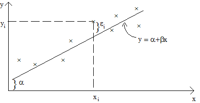
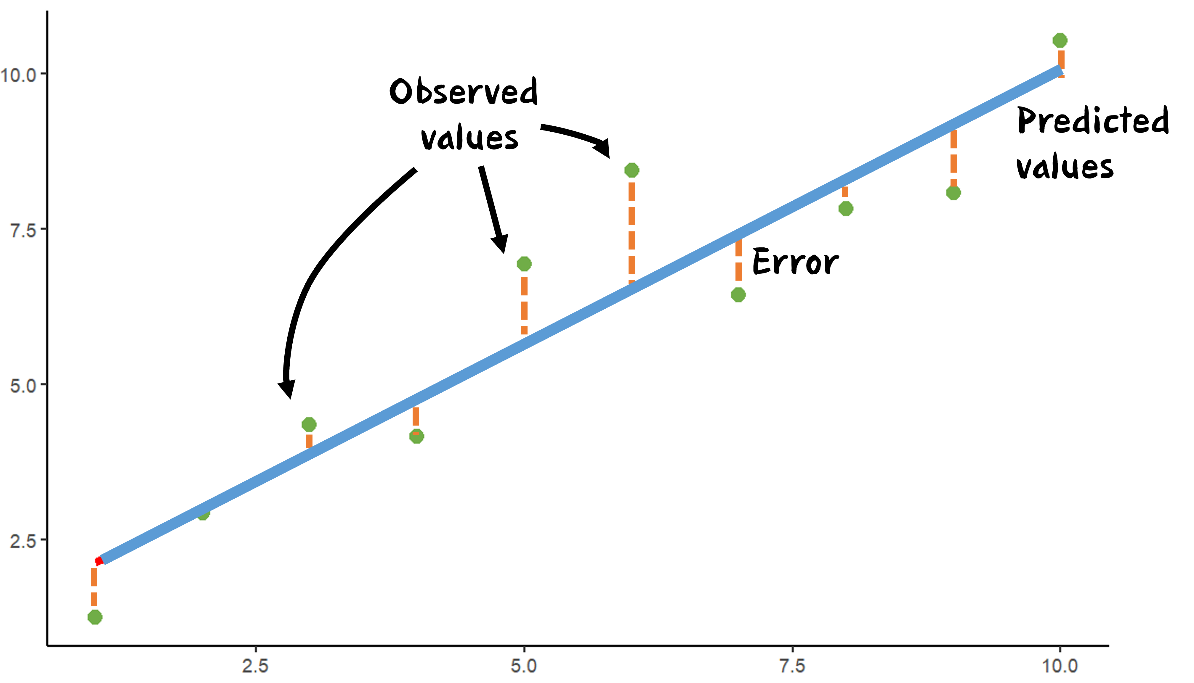
By fitting this line to our data, we can make predictions (also called “fitted values”) for the 'x' values in the data set. The difference between the predicted 'y' value and the actual 'y' value for a data point is called the residual and often denoted by \( \epsilon \).
Estimating Parameters
.....
In SLR, we deal with two unknown parameters: the slope and the intercept. We estimate these values using a method called least squares. The idea is to find estimates that minimise the residuals, thereby improving the model's fit to the data. A GIF (right) illustrates how changing the regression line can minimise the "squares".

Extra Resources: What are Least Squares?
Interpreting Output
When we run an SLR analysis using statistical software, we typically get two main outputs:
Model Coefficients Table:
This table gives us estimates for the slope and intercept of the regression line. The table also allows one to make inferences concerning the slope of the regression line. A t-test is used to test the hypothesis that there is no linear relationship i.e. slope, \( \beta = 0\). In practice, just the computer output \(P>|t|\), will be interpreted. This is the p-value for the test.
ANOVA Table:
This table breaks down the overall variation in 'y' into two parts:
- Variation due to the regression, i.e. due to the presence of the explanatory variable, \(x\).
- The leftover variation, which isn't explained by the 'x' variable.
Extra Resources: ANOVA tables

Quiz: Accounting for Variability
-
-
-
The error term, also known as "residuals," represents how much the actual data points differ from the ones predicted by our model. It helps us see the parts of the data that our model has not accounted for.
By examining the distribution of these errors, we can better understand how well our model is doing.
When we study the error distribution, we're essentially asking two questions: Can we improve our model to account for more of the variability in the data? And, are there parts of the data that our model still does not account for?
For additional information on residuals, or a refresher on results, there are a set of slides given in the box below:

Resources: What are Residuals?
Linking to this, there is a mastery quiz on residuals that be accessed in the box below:

Quiz: What are Residuals?
-
-
-
File
-
Quiz
-
-