Variation & standard deviation
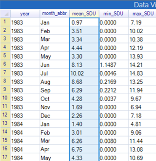
Climatic data are variable. With rainfall data, some days are dry, i.e. zero rainfall, while others have large amounts of rain. Temperatures fluctuate, both within the day and between days. In the example shown here, we have daily and monthly sunshine data. Just from the first few rows of the daily data we see some days have no sun (zero values) while others have sun.
It is useful to have summary values for the variation in the same way as the mean, minimum and maximum are summaries of location. The most commonly used summary is the standard deviation (which is the square root of the variance). The COMET course called Introduction to Statistics for Climatology gives the formula and shows the calculation, for those who find this useful. Here we assume your software will do the calculations, so we concentrate on its interpretation and use.
Our initial data, as before, are the daily and monthly sunshine records:
| Daily sunshine hours | Monthly summaries from the daily data |
|---|---|
 |
 |
It is easy to calculate any summaries you wish, but they are not always useful. Start with the daily data. The minimum for the sunshine is clearly 0, and the maximum will be a completely sunny day. For Frankfurt the maximum day length is just less than 17 hours, so calculating the maximum from the data of 16.2 hours, seems both reasonable and obvious. That is useful to calculate, if only to check that it is not longer than the longest day length.
The mean will be roughly in the middle. Do you think it is likely to be more, or less, than 8 hours (halfway between the minimum and maximum?) And roughly how large to you think the standard deviation is?
Is it roughly
- 1 hour,
- 5 hours,
- 12 hours,
- 25 hours,
- 144 hours, or
- Impossible to say?
Calculate it first.
Well the standard deviation is sort of a typical distance from the middle. If the middle is 8hrs sunshine per day, then the maximum distance from the middle is 8 hours (either 0 or 16), and hence a typical – unsurprising distance is 4 hours.
The exact answer is calculated as 4.4 hours. So the simple idea is that the standard deviation is roughly a quarter of the range. Usually it is, as in this case, slightly larger than that.
The data are skew, and the mean is 4.9 hours per day, partly because you can have zero or small values right through the year, but large values, more than 12 hours are limited to the summer months. However, more important, is the notion that reporting the mean as 4.9 hours is a useful summary, but there is no real value in knowing that the standard deviation of these daily data is 4.4 hours.
So why might the mean be useful? If the mean, from the daily data, is 4.94 hours, then, in a year, there is an average of 4.94 * 365.25 = 1804 hours of sun. So, with solar energy, that could be a useful figure to evaluate, on average, roughly the electricity to be generated.
So why do we claim the standard deviation of the Frankfurt daily data isn’t useful in the same way? To help with the answer we first calculate a standard deviation that could be useful. We have the monthly summary data for Frankfurt and use it to calculate the annual totals. The results are shown below.
Now calculate the summaries from these total values. The mean is 1804, as before1. The minimum is 1543 hours, and the maximum is 2255 hours. So, we expect the standard deviation to be close to ¼ of the range, so close to 178. The calculated value is 145hrs2. This could be a very useful summary of the amount of variation in the solar energy from year to year.
| First lines from monthly sunshine data | Annual totals |
|---|---|
 |
 |
These data are all time series. The analysis of time series often starts by splitting the data into the trend, the seasonality and the residual. There is a lot of seasonality in the Frankfurt sunshine data, and hence the standard deviation of the daily data is a mixture of the known variation (mainly seasonality and the unknown residual variation. The annual data above, has got rid of the seasonal effect. For the monthly data, we could also find useful standard deviations by analysing each month separately.
Variation of the data. Useful to understand what the standard deviation is all about. But need to take out the variation you know about – seasonal variation. Variation within the season. Variation of daily values in the month.
1 The fact that the sum of the (daily) means is the same as the mean of the annual totals is another attractive property of taking means. You can’t do the same with medians or other percentage points.
2 So, it is roughly a quarter of the range, but, from the rough “rule of thumb” we might have expected the standard deviation to be slightly larger – or the range to be smaller. When there is a surprise, it is usually useful to examine individual values. Here we see the largest value, in 2003, of 2255 hours is much larger than the second highest - which is 2041 hours, and is the only other year with more than 2000 hours. Without the 2255, a quarter of the range would be 125 hours – so a bit less than the standard deviation. Investigating further we find that June to August 2003 is remembered as having a serious heatwave.